When data are not so informative, it pays to choose the sum score over the factor score

When I first came across the recent preprint by McNeish and Gordon Wolf on Twitter on how sum scores are factor scores from a heavily constrained model, my first reaction was: don’t we all know this already? Sacha Epskamp asked the same question and there’s a discussion that follows about how people who study these topics know this, but applied researchers may not.

I skimmed the paper and the authors show how sum scores are factor scores when all item error variances are the same and all loadings are the same across items. This is a highly constrained model; fwiw, it’s no different conceptually from the widely used Rasch model. And the authors argue that it’s important to justify this sum score model. They also admit that in many situations, it makes no practical difference which score you use. And they point out that differences between both scores will exist when the loadings are different across items.

Now, although I think the difference between the sum score and factor score is of importance, what is more important is the relationship any of these scores have with the latent trait (assuming such a thing exists). Another widely known fact is that any score from these models differs from the latent trait such that the correlation of these scores to the latent trait is less than one. This is why there is a new line of research by Ines Devlieger (reviving an older line of research) on how to properly use factor scores in models while accounting for the fact that the score is not the trait.¹²

Another feeling I had in reaction to the paper is that small sample sizes are quite common in applied research settings and a researcher is probably better off working with the sum score when their sample size is small.³ Although the CFA may return unbiased estimates of the relationship between items and the factor when the model is true, at small sample sizes, such estimates are likely to be unstable such that a crude guess like: “a factor loading of 1 for each item” i.e. sum scoring will be better. This is the bias-variance trade-off.⁴

So I decided to test this issue empirically, my hypothesis being that the sum score will be better related to the latent trait under small sample sizes. After testing, the short answer is:

When the data are not so informative (e.g. small sample + weak loadings), the sum score is better than the factor score.

Here’s how I went about:

The sim.fun() function takes a latent variable, lv; a set of loadings, lambda; and the number of times to replicate a simulation and analysis. The first step is to generate multivariate normal data according to the standard CFA formula: \(\mathbf x = \boldsymbol{\Lambda\xi} + \boldsymbol{\delta}\); basically, multiply loadings by latent variable and add error. I wrote the code such that the error variance for each item = 1 - loading ^ 2 for the item. Hence, one can think of the loading squared as the proportion of variance in the item that is accounted for by the latent variable. The final analysis in the function is to compute sum scores, factor scores from a standard unidimensional CFA and coefficient alpha. The function then returns coefficient alpha, and the correlations of sum and factor scores to the supplied latent variable. I repeated this 2,000 times for five sets of loadings:

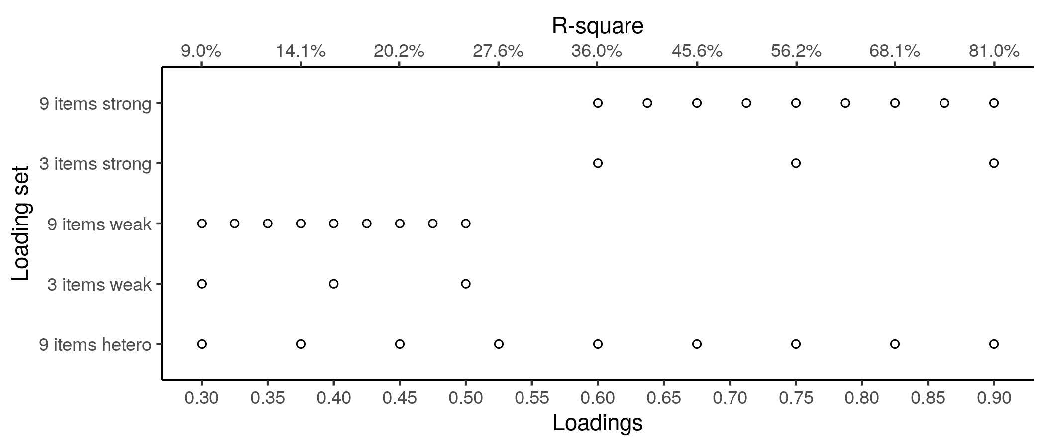
The latent variable was always a rankit score of sample size 60, hence, very close to standard normal.

I assumed any difference from 1 in the correlation between the scores and the latent variable represented bias, and I calculated the mean squared error to assess estimation quality. I know both scores are somewhat different from the latent variable, so the correlations will generally be under one. I used the absolute value of the correlation of the factor score and latent trait in all calculations.⁵ Here’s what the MSEs look like:

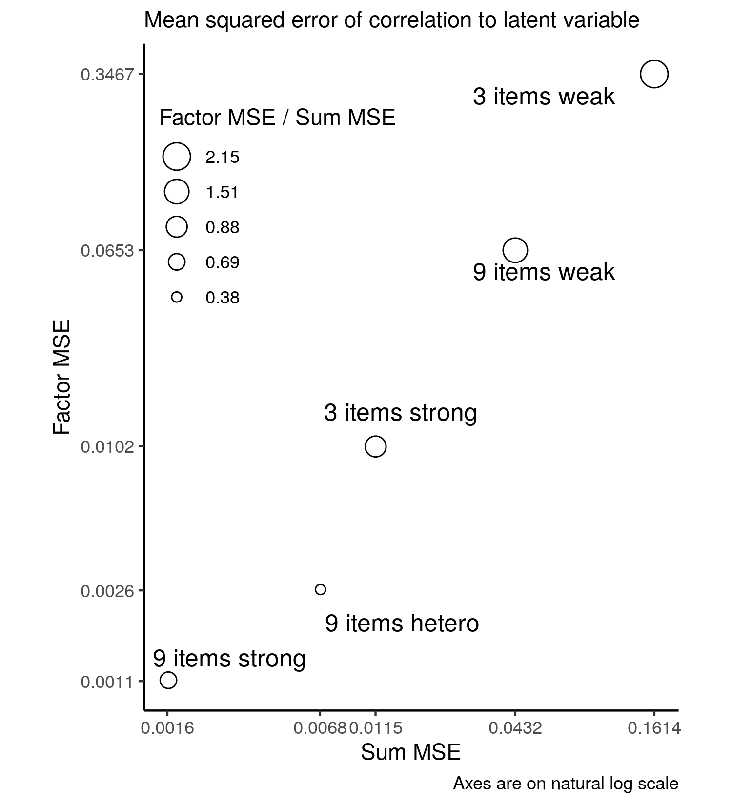
It’s clear that under weak loadings, whether with 9 or 3 items, the sum score is much better correlated to the latent trait than the factor score. To get a better sense of what the correlations are, another plot:

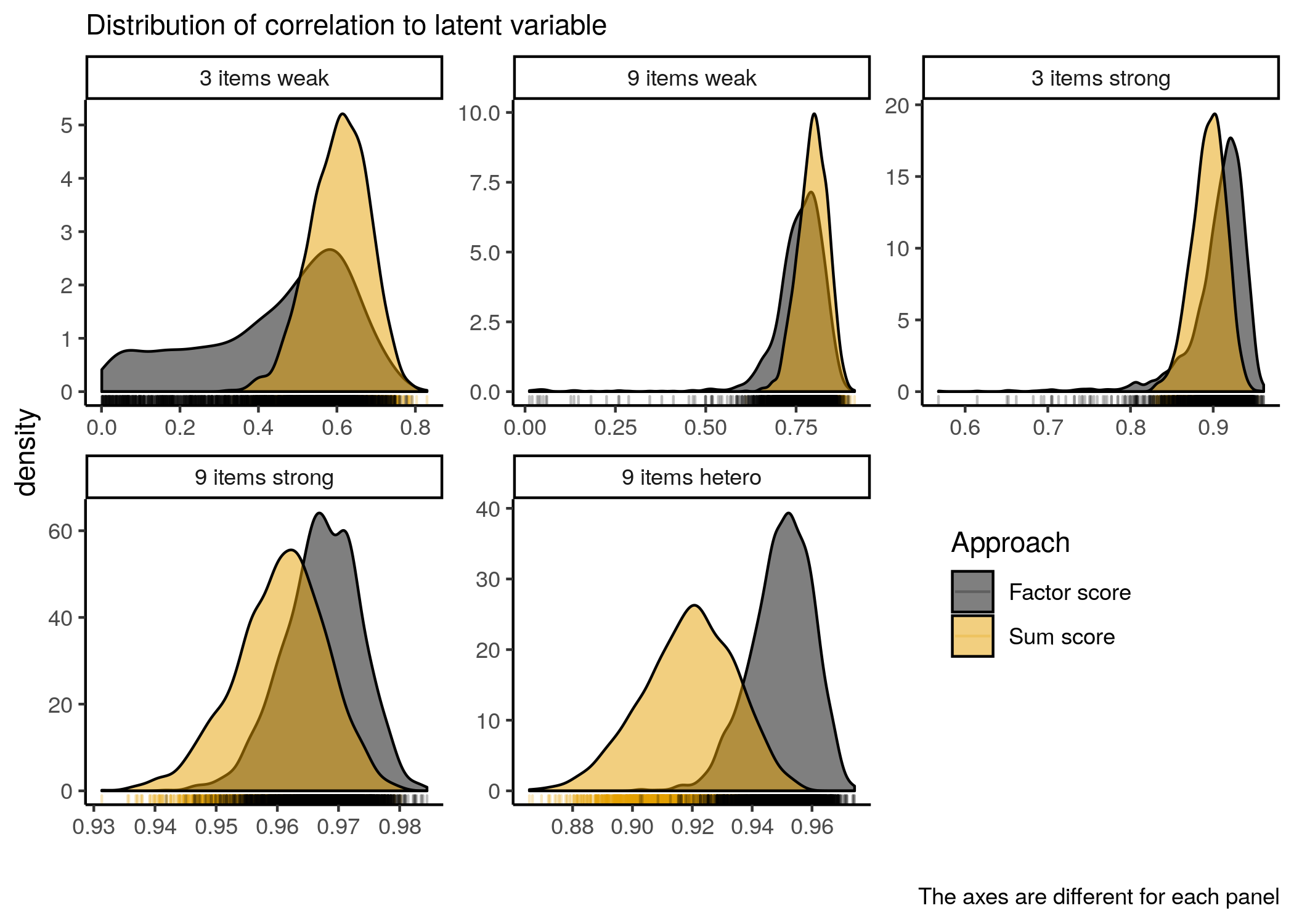
We see here that when the loadings are weak, the correlation of the factor score to the latent trait has a very wide range relative to the same correlation for the sum scores. When the loadings are strong, the situation is reversed. Under the heterogeneous condition, the factor score is clearly better.

But even when the loadings are strong, the relationship of the sum score to the trait is not much different from the relationship of the factor score to the trait. Moreover, when there are only three items, one still finds some low correlations (.5, .6, .7) when using the factor score approach - see black spikes under plot in 3 items strong panel.

One of the key recommendations of the paper by McNeish and Gordon Wolf is to validate the sum score model. The easiest way to do this is to perform the CFA with loadings constrained equal and error variances constrained equal i.e. the sum score model and test it. Remember, this model like all models is always wrong.⁶ But if there is insufficient statistical power to detect the misspecification of this model, there is probably insufficient information in the data for more complicated modeling. So I also performed \(\chi^2\) testing of the sum score model across replications:

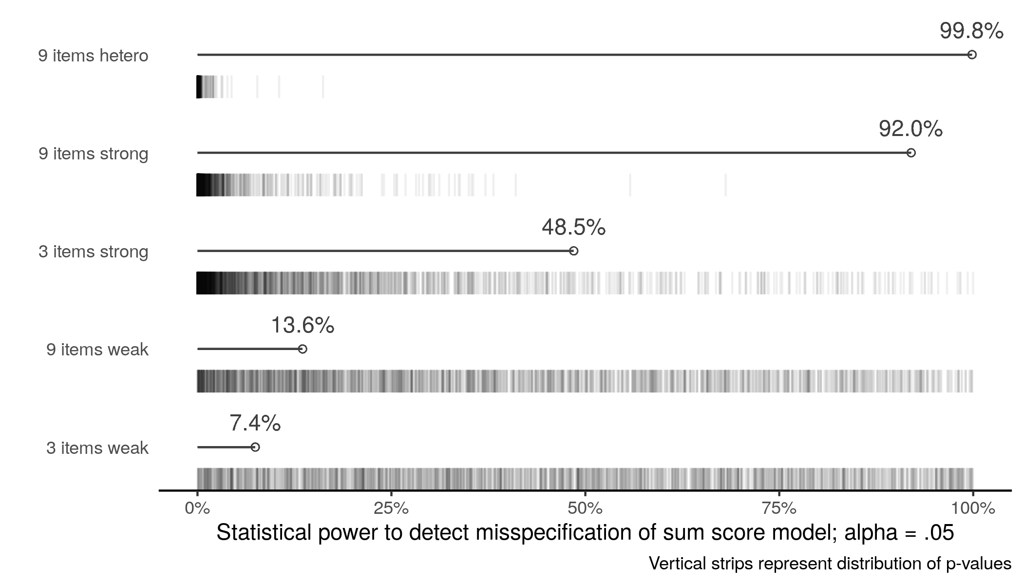
This plot is consistent with the rest of the text. But we should note that even when there is power to detect misspecification of the sum score model, the sum scores are still similarly correlated to the latent trait as the factor scores.

In all, nothing here is new. None of these models will ever be correct for data. When data are uninformative, simple crude approaches like a sum score will do the job and may be better than more complicated modeling, unless the more complicated modeling is a well-done Bayesian analysis.