The limitations of small variance priors lie in their implementation

Thanks to Muthén & Asparouhov (2012), hereafter MA2012,¹ small variance priors are a common feature of Bayesian SEMs. The idea is: when we are not sure that a parameter is zero, you can place a prior that attempts to constrain the parameter to zero. A non-zero parameter will hopefully escape the constraint, while zero parameters will have most of their posterior concentrated around zero.

Estimation of parameters constrained to zero

In latent variable models, we assume relations between observed items are captured or mediated via the latent variables. Assuming we have six items, we may assume the first three reflect latent variable 1, and the second three items reflect latent variable 2. The first three items have non-zero loadings on latent variable 1 and zero loadings on latent variable 2. And the second three items have zero loadings on latent variable 1 and non-zero loadings on latent variable 2.

We assume the individual items may be correlated only because they either reflect the same latent variable or the different latent variables they reflect are correlated. In our example, if latent variable 1 and 2 have zero correlation, then items 1–3 should have no correlation to items 4–6.

In practice, data tend to deviate from these clean hypotheses:

1. Items may be residually correlated beyond the correlations implied by their latent variables relations and the items relations to the latent variables. For example, items 1 and 4 may share similar wording that induces respondents to respond to them similarly beyond what the latent variable relations imply.
2. Items may reflect latent variables we hypothesized them to be unrelated to. For example, item 3 may reflect the second latent variable in addition to reflecting the first latent variable.

To address these possibilities, one can place a small variance prior on all residual (cor-)relations between items, or on all loadings assumed to be zero. If any of these parameters are notably large, we should be able to identify them from their resulting posterior distributions.

Small variance priors also show up in differential item functioning / measurement invariance analysis. There, we can place such a prior on the difference in a parameter across groups. If the difference is large enough, it should escape the constraint induced by the prior, suggesting differential functioning/non-invariance.

Jorgensen & Garnier-Villarreal, 2023

Jorgensen & Garnier-Villarreal (2023), hereafter JGV2023,² assess the ability of small variance priors to deliver on these promises and find them wanting. I will focus on their first simulation study.

Estimating a missing cross-loading

JGV2023 set up a six-item problem like in the example above, first three items reflect latent variable 1, second three reflect latent variable 2, all loadings are 0.7, latent variables are correlated at 0.25 and total variance of each item is 1.

They also assume that item 3 may reflect latent variable 2, they vary the value of this cross-loading (which we will call L3,2) as a simulation condition: 0, 0.2, 0.5, 0.7.

Ideally, a small variance prior applied to all cross-loadings should identify this parameter as non-zero when L3,2 is not zero. They follow guidelines in MA2012: if the 95% interval on the parameter includes 0, they decide the approach has failed to detect that this cross-loading is non-zero.

First, they find that this approach does not really improve over using modification indices to identify what changes to make to a model, i.e. add L3,2 to the model as a pre-specified parameter.

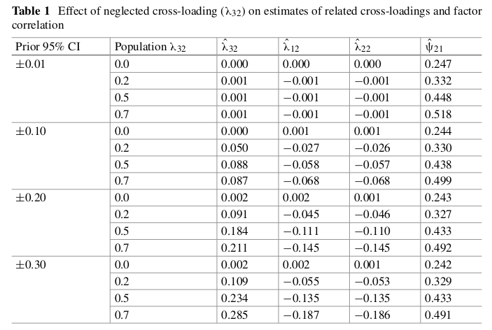
They also track the estimated value of L3,2 and find that the estimated value is much lower than its true value using small variance priors.

A related problem is: assuming a non-zero cross-loading is zero inflates the (cor-)relation between factors. So they track the estimated value of the correlation between both latent variables when using small variance priors on cross-loadings, and find this relation to be well above the correct 0.25. This value is sometimes as high as 0.5 when the true value of L3,2 is 0.7.

The results are bad, see a screenshot of Table 1 in their paper.

I will now discuss some issues I have with small variance priors as implemented.

How small should the variance in my small variance prior be?

This is one challenge with implementing small variance priors. Small variance priors usually take the form: \(\mathcal{N}(0, \sigma)\), where \(\sigma\) is small relative to the scale of the parameter.

Assuming observed items have an SD close to 1 and latent variables are assumed standardized, loadings are akin to standardized regression coefficients in their scale. They tend to be larger than typical standardized regression coefficients, and salient loadings will tend to vary between 0.4 and 0.9 with 0.7 as a typical expected value.

So a weakly informative prior on a loading might be: \(\mathcal{N}(0, 1)\) which assumes 95% chance the loadings lies between -2 and 2.

A small variance prior might then be: \(\mathcal{N}(0, \sigma = 0.05)\) which assumes that loadings will mostly fall in the (-0.1, 0.1) interval.

Different choices of \(\sigma\) will have different impacts on the resulting posterior distribution of the parameter that has a small variance prior placed on it. And Asparouhov, Muthén & Morin (2015) recommend varying \(\sigma\) as a kind of sensitivity analysis.³

JGV2023 used four values of \(\sigma\) as one of their simulation conditions: 0.005, 0.05, 0.10, 0.15.

This general approach is my first issue with the common implementation of small variance priors. A Bayesian solution is to learn the size of \(\sigma\) from the data, by placing a prior on \(\sigma\) – some citations within Bayesian SEM of this kind of practice.⁴

It would correspond to fairly standard Bayesian regularization / hierarchical modeling.

Choice of distribution of small variance priors

Another issue is the choice of distribution. Priors correspond to beliefs about parameters. The degree to which the belief is incorrect will determine the degree to which the model is insightful.

In the data generation process for JGV2023 (and in most model misspecification studies), researchers create misspecification by assuming a clean model, but the estimated model fails to incorporate a non-zero parameter. In this example, the mistake is to ignore the cross-loading of item 3 on latent variable 2. I personally don’t think this is a realistic model of misspecification, preferring random models of misspecification; see Wu & Browne (2015)⁵ and the Uanhoro citation in ⁴.

But let’s work within this framework, all missing cross-loadings are zero, except for one of them. The distribution of these cross-loadings is definitely not normal. A small variance normal prior assumes that cross-loadings are on average zero, with varying gradations away from zero, no outliers. This assumption is generally realistic for misspecification that occurs in practice, but does not match the way SEM researchers generate misspecification.

A prior that matches SEM researchers' model is one that assumes parameters are mostly zero with a few non-zero parameters. Several distributions attempt to approximate such an assumption: double-exponential (lasso),⁶ (regularized) horseshoe,⁷ generalized double-Pareto (GDP),⁸, …

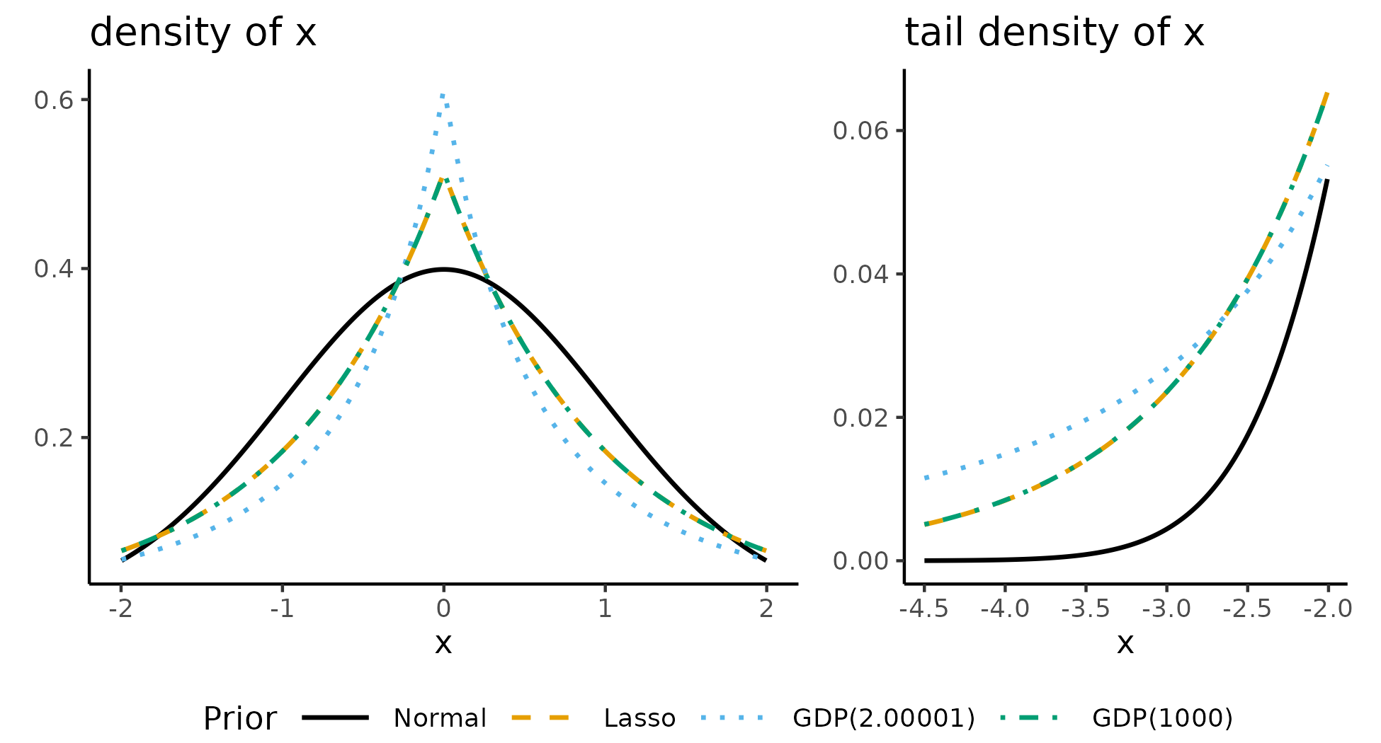
As shown in the plot above, these alternatives to the distributions have a spike at zero, and heavy tails – they expect a couple large outliers. All distributions in the plot above have the same interquartile range. Yet we see that the lasso and GDP are expectant of outliers with since both distributions have larger tail densities than the normal distribution.

When the GDP shape parameter is large (GDP(1000)), it matches the lasso distribution. When the GDP shape parameter is small (GDP(2.00001)), it has a larger spike around zero suggesting greater shrinkage of small parameters to 0 and is more expectant of outliers, suggesting less shrinkage of large parameters.

Under these priors, the mode of the posterior distribution of zero parameters will be zero, and the posterior mode for non-zero parameters will be non-zero.

I do not think these priors reflect my beliefs about misspecification. Models in practice tend to have several small-ish but non-zero missing parameters and a few larger missing parameters, matching the normal prior assumption or maybe a t-distribution.

But simulation studies generate perfectly clean data, and the misspecification is due to the researcher’s ignorance of one or two missing parameters. Well, if researchers generate data under such assumptions, then the priors should match these assumptions.

Even if one believes the more realistic pattern of misspecification, one can – for pragmatic reasons – assume a spike-at-zero-heavy-tail distribution to separate small misspecifications from larger misspecifications. The small missing parameters will have posterior modes of 0, and the non-small missing parameters will have a non-zero posterior mode.

This forms the basis of my attempt at repeating study 1 in JGV2023.

Repeating JGV2023

I repeat the study, but use a generalized double-Pareto prior on cross-loadings. Like JGV2023, I varied sample size between 50 and 1000.

The parameters of the GDP prior were learned from the data. This feature is implemented in the minorbsem R package – a Bayesian SEM package I created to estimate models like this. I have shared the simulation code as a gist:

I review the results from the study.

Examining posterior modes

First, I track the posterior mode of all cross-loadings. We can expect the posterior distribution of the cross-loadings of items 1 and 2 on latent variable 2 to be impacted by the presence of a non-zero cross-loading of item 3 on latent variable 2. So I track three sets of cross-loadings:

1. Item 3 on latent variable 2 – focal cross-loading
2. Items 1 and 2 on latent variable 2 – JGV2023 found them to be non-zero and negative when using small variance priors
3. Items 4 – 6 on latent variable 1 – these cross-loadings should be minimally impacted

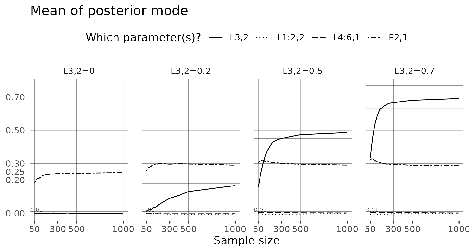
The results are below:

There are four panels, each panel represents a true level of L3,2. In the leftmost panel, L3,2 is 0. In the rightmost panel, L3,2 is .7.

The solid line represents the posterior mode of L3,2 and we find that on average, it is distinctly different from all other loadings. As sample size increases, it closely approximates the true parameter.

We also find that the average posterior mode for all other cross-loadings is less than 0.01.

This result is different from JGV2023’s where the cross-loadings of items 1 and 2 on latent variable 2 were negative on average and L3,2 was much smaller than its true value on average.

The plot also reports the average correlation between the latent variables, ideally, 0.25. We consistently estimate an upwardly biased correlation of about 0.3. This result is nowhere as problematic as JGV2023’s results which saw this correlation approach .5 in certain conditions.

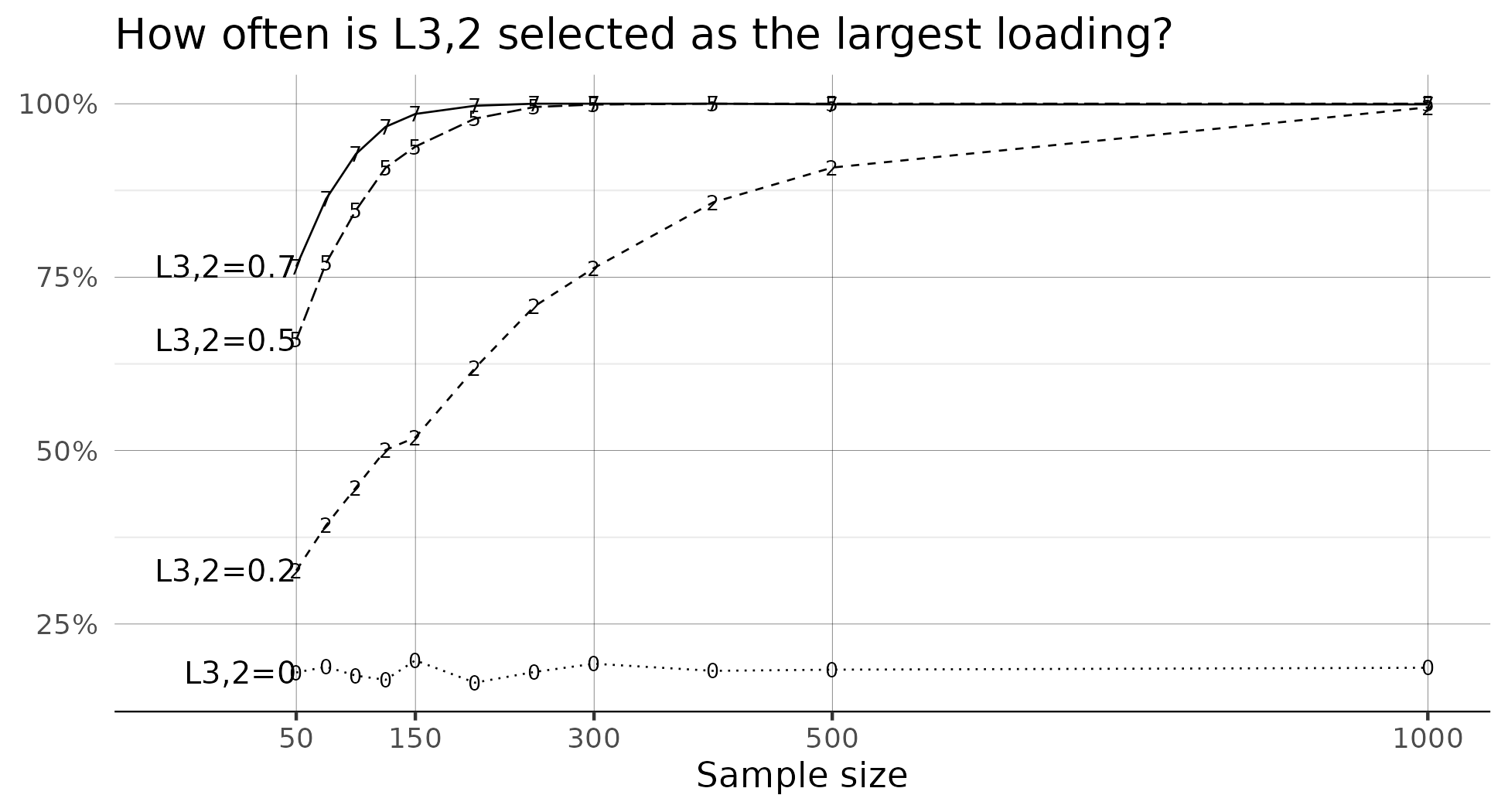
How often does the model identify L3,2 as having the largest cross-loading?

This plot shows that the model does a fairly good job of identifying L3,2 as having the largest cross-loading. When L3,2 is 0.5, the model identifies this parameter as having the largest cross-loading more than 60% of the time when the sample size is 50. By sample size of 125, the model identifies this parameter as having the largest cross-loading more than 90% of the time.

In summary

My hope is that these results show that the right type of small variance prior lives up to its promise. A big part of the problems shown by JGV2023 stem from the inadequacy of the specific small variance prior to the specific problem.

Part of the issue here is that the average Bayesian SEM user (i.e. not JGV) uses Mplus. And as far as I can tell, Mplus only permits the normal distribution for small variance priors and the variance has to be fixed a-priori. This limits the models we see in practice.

Allowing more flexible small variance priors where the prior scale (and maybe shape) is learned from the data is not so hard to implement. Hopefully, we can see something like this in blavaan in the future.

Holzinger-Swineford example

I conclude with the Holzinger-Swineford example and assume the first three, second three and final three scores reflect the first, second and third latent variables respectively.

When I estimate all cross-loadings using a generalized double-Pareto prior, the posterior modes of the resulting cross-loadings are:

       [,1]  [,2] [,3]
 [1,]    NA  0.18 0.00
 [2,]    NA -0.01 0.00
 [3,]    NA  0.00 0.00
 [4,]  0.00    NA 0.01
 [5,] -0.02    NA 0.00
 [6,]  0.02    NA 0.00
 [7,]  0.00  0.00   NA
 [8,]  0.00  0.00   NA
 [9,]  0.32  0.00   NA

Only two parameters, the cross-loading of item 1 on the second latent variable and the cross-loading of item 9 on the first latent variable, escape the constraint.

We can estimate a final model with both parameters included.

The code for this example is:

library(minorbsem)

writeLines(base_formula <- paste(
  paste0("F1 =~ ", paste0("x", 1:3, collapse = " + ")),
  paste0("F2 =~ ", paste0("x", 4:6, collapse = " + ")),
  paste0("F3 =~ ", paste0("x", 7:9, collapse = " + ")),
  sep = "\n"
))

mod_base <- minorbsem(
  base_formula,
  data = HS, method = "none", seed = 1
)

mod_crossload <- minorbsem(
  base_formula,
  data = HS, simple_struc = FALSE, method = "none", seed = 1
)

# produces a warning
load_modes <- apply(
  posterior::as_draws_matrix(mod_crossload@stan_fit$draws("Load_mat")), 2,
  modeest::hsm
)
post_mode_mat <- matrix(load_modes, 9)
post_mode_mat[mod_crossload@data_list$loading_pattern != 0] <- NA_real_
round(post_mode_mat, 2)

mod_simp <- minorbsem(
  paste(
    base_formula,
    "F1 =~ x9", "F2 =~ x1",
    sep = "\n"
  ),
  data = HS, method = "none", seed = 1
)